Example 1: Multiple Regression

This example is based on the data file Poverty.sta, which contains data for a comparison of 1960 and 1970 Census figures for a random selection of 30 counties. The purpose of this study is to identify the factors that correlate with the percent of families below the poverty level in a county (Pt_Poor), and to build a predictive model for that variable. Thus Pt_Poor will be treated as a dependent (response) variable, and the other 6 variables as continuous predictor variables.

Ribbon bar. Select the Home tab. In the File group, click the Open arrow and select Open Examples to display the Open a STATISTICA Data File dialog box. Open the data file, which is located in the Datasets folder. Then, select the Statistics tab. In the Advanced/Multivariate group, click Advanced Models and from the menu, select General Partial Least Squares to display the Partial Least Squares Models Startup Panel.

Classic menus. From the File menu, select Open Examples to display the Open a STATISTICA Data File dialog box. Open the data file, which is located in the Datasets folder. Then, from the Statistics - Advanced Linear/Nonlinear Models submenu, select General Partial Least Squares Models to display the Partial Least Squares Models Startup Panel.

Select Multiple regression as the Type of analysis, Quick specs dialog as the Specification method, and click the OK button to display the PLS Multiple Regression Quick Specs dialog box.

Click the Variables button to display the standard variable selection dialog box. Select PT_POOR in the Dependent variable list, select all other variables as the Predictor variables (covariates), and then click the OK button.

The PLS Multiple Regression Quick Specs dialog box will now look like this.

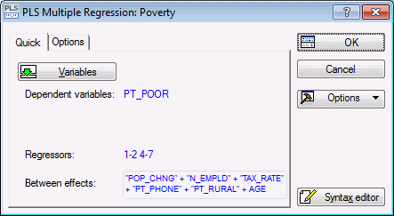
For this example, we will accept all other defaults, so click the OK button to begin the analysis and display the PLS Results dialog box.

If you want to run this example using PLS Syntax, you can run the following syntax program from the PLS Analysis Syntax Editor (see Methods for specifying designs).

Reviewing Results Summary

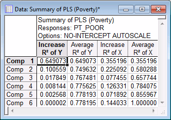
On the PLS Results - Summary tab, click the Summary spreadsheet button to produce a spreadsheet as shown in the following image.

You can visualize these results by clicking the Summary graphics button.

The spreadsheet shows the R-square values and R-square increments for the respective number of components, listed in the rows. The R-square values are computed for the predictor variables (columns in the design matrix; the respective spreadsheet column is labeled R2 of X) and the dependent (response) variable (the respective spreadsheet column is labeled R2 of Y). The average R-square value for the predictor (X) variables is computed as the averaged R-square over the predictor variables (columns in the design matrix); the average R-square value for the Y variables (there is only one Y variable in the present analysis) is computed analogously. Also, unlike in STATISTICA General Linear Models (GLM) or Multiple Regression, the R-square values are computed relative to the sums of squared deviations from the origin (0.0) for the centered (de-meaned) predictor variables (columns in the design matrix) and dependent (response) variable. So the results will not be identical to those computed in, for example, GLM or Multiple Regression.

The pattern of R-square values over the number of components will allow you to decide how many components to retain for the remainder of the analysis. In this example we will retain two components, since there appears to be a leveling off of the R-square value for the dependent (response) variables at that point (see the R2 of Y values).

Weights for X

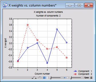
Next, click the Weights for X spreadsheet button.

The spreadsheet shows the weights for the predictor variables, i.e., the contribution of each predictor to the respective component (the W weights; for details about these weights, and the computations performed in the PLS analysis, see also Computational Approach).

You can reduce or increase the total number of components that are being considered via the Number of components field. For example, shown below is the plot of the Weights for X for 2 components (enter 2 in the Number of components field, and then click the Weights for X graphics button.)

These results show that variables Pop_Chng (population change), Pt_Phone (percent of residences with telephones), and Pt_Rural (percent of rural population) are the most important contributors to component 1, and hence to the model which explains approximately 65% of the variability of the dependent (response) variable Pt_Poor (i.e., the R2 of Y in the Summary of PLS spreadsheet is .649).

Loadings

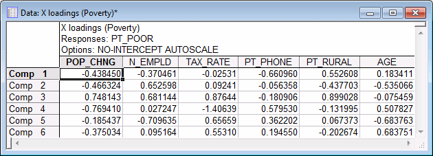
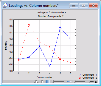
Next, reenter 6 in the Number of components field and then, on the Summary tab, click the Loadings spreadsheet button.

This spreadsheet shows the factor loadings (P; see the description of the computations in Computational approach). Once again, you can reduce or increase the total number of components that are being considered via the Number of components field. For example, shown below is the plot of the Loadings for 2 components.

These results indicate that variables Pt_Phone (percent of residences with telephones) and Pt_Rural (percent of rural population) are the most influential variables that define component 1, and hence the model that explains approximately 65% of the variability of the dependent (response) variable Pt_Poor (i.e., the R2 of Y in the Summary of PLS spreadsheet is .649).

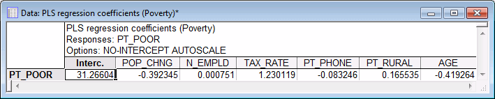
PLS Regression Coefficients

Next, reenter 6 in the Number of components field and then, on the Summary tab, click the Regr. Coeffs spreadsheet button.

Note: the No intercept option on the PLS Quick Specs dialog box - Options tab affects the linear combinations that create the new components. The option does not affect the regression equation, as can be seen to contain an intercept.

The values in this spreadsheet are the unscaled regression coefficients, so they can be used to compute predicted values for new data. Each row of the spreadsheet represents the regression coefficients corresponding to each response variable; in this example, of course, we only have a single response variable (Pt_Poor).

Again, you can reduce or increase the total number of components that are being considered via the Number of components field. Shown below are the plots of the Regr. Coeffs for 2 and 6 components, respectively.

 

It appears that the regression coefficients computed from 2 components or from 6 components are very similar to those that can be computed via ordinary Multiple Regression. However, PLS regression coefficients are usually more robust (Geladi and Kowalsky, 1986).

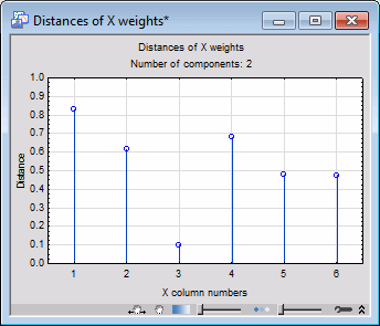
Another Plot of Weights

Let's produce another plot of the X weights, for 2 components. Once again enter 2 in the Number of components field, select the Distances tab, and then click the X weight dist. graphics button.

The values plotted in this chart are the Euclidean distances of the predictor variables (effect columns) from the origin computed from the X weights over the current number of components (2). Specifically, each distance is the square root of the sum of squared X-weights over the current number of components. Clearly, columns 1 and 4 (in the design matrix; i.e., variables Pop_Chng and Pt_Phone, use the Design terms button on the Summary tab to review the relationship between the columns in the design matrix X and the original predictor variables in the analysis) show the largest distances, and are thus the major contributors to the prediction of the conceptual variable Poverty (variable Pt_Poor).

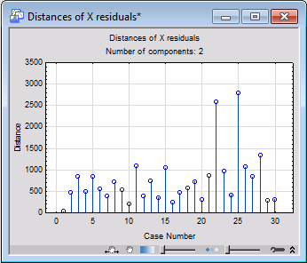
Observational Statistics

Another plot of interest on the Distances tab is the plot of the X resid. dist. This graph is shown below.

This plot shows the Euclidean distances of the observations from the origin computed from the X residuals over the predictor columns (in the design matrix), for the current number of components (2). It appears that observation 25 (Shelby county) shows an unusually large residual value, and therefore may be an outlier that you may want to exclude from the analysis.

Next, select the Observational tab to review the predicted and residual values for each observation. On this tab, you can review various plots and spreadsheets of predicted and residual values for both the predictor columns (in the design matrix) and the dependent (response or Y) variable. Careful examination of these results will provide further evidence that observation 25 may be an outlier that has a disproportionate influence (relative to the other observations) on the results obtained in this analysis.

See also, PLS - Index.