SANN Example 6: Deploying the 4Bar Linkage Data
This example illustrates how to deploy saved PMML files and reviews some of the options that are available during deployment. It uses the PMML files that were saved as part of Example 1: Performing Regression with the 4Bar Linkage Data. It is necessary to complete that example before beginning this one.
Note: The results shown here might be slightly different for your analysis because the neural network algorithms use random number generators for fixing the initial value of the weights (starting points) of the neural networks, which often result in obtaining slightly different (local minima) solutions each time you run the analysis. Also note that changing the seed for the random number generator used to create the train, test, and validation samples can change your results.
Deployment
In order to deploy a saved network, you must have a data set (or Streaming DB Connector) opened in Statistica. This active data set must contain the same inputs as the saved network. Although you ordinarily would not deploy a network with the same data that was used for training, however, for this example this is done.
- Open the 4Bar linkage.sta data file that is distributed with Statistica in the Examples/Datasets subfolder of your installation.
- In a real deployment situation, it is unlikely that target variables would be available. You can simulate that situation by deleting the target variables from this data set. Select the columns for T3, T4, H1, and V1, then right-click in the variable header and select Delete Variables.
- The Delete Variables dialog box is displayed.
- Click the OK button to remove these four variables from the active data set.
- Save the data set to your desktop as 4bar deployment.sta using of the following ways.
- Start SANN using one of the following ways:
- Ribbon bar: Select the Data Mining tab. In the Learning group, click Neural Networks to display the SANN - New Analysis/Deployment Startup Panel.
- Classic menus: From the Statistics menu or the Data Mining menu, select Automated Neural Networks to display the SANN - New Analysis/Deployment Startup Panel.
- In the Deployment group box, select the Deploy models from previous analyses option button. Then, click the Load network files button. From the Open dialog box, locate the two files saved at the end of Example 1 (4barlinkage-1.xml and 4barlinkage-2.xml), and open them. The SANN - New Analysis/Deployment Startup Panel will now display the saved networks (note that your networks may vary).
- When a network file is opened for deployment, the analysis type is automatically selected in the New analysis list box. As shown, Regression is selected. If you had opened a time series (regression) network, then Time series (regression) is selected.
- When multiple network files are selected for deployment, SANN opens them in this way: SANN reviews the inputs in the first file and verifies that the input variables are available in the active data set. If the inputs are not available in the active data set, the network is not opened. Once a network is opened, SANN scans the next file to verify that the same inputs are used in both files and that the analysis type is the same. If both networks contain the same inputs and use the same analysis type, then the second network is opened, and the next network is scanned. This process continues until all selected networks are reviewed. All networks that contain the same inputs and analysis type as the first opened network will be opened; any other networks are discarded for the analysis. At the end of this process, SANN informs you if some networks cannot be opened.
- Click the OK button to display the SANN - Data selection dialog box - Quick tab. The options in this dialog box are the same as during training; however, for deployment, they are dimmed. You are able to review the variables that have been selected, but you cannot modify variable selection.
- Select the Sampling (CNN and ANS) tab.
- The Quick tab has options that are the same as during training; however, their use is slightly different. Because no training takes place during deployment, options for specifying a training subset or a validation subset are dimmed. During deployment, all cases are treated as test (or deployment) cases. You could choose to limit the cases that are deployed using the options in this dialog box. For example, if you only want to deploy 80% of the cases in the active data set, you would select the Random sample sizes option button and set the Test sample size % field to 80. Only 80% of the cases in the active data set would be deployed. You could also use a sample variable to specify which cases are deployed. To do this, you would select the Sampling variable option button. The Testing sample button would be activated, enabling you to select the variable that indicates which cases should be deployed. The control for selecting the variable and code are identical to those used in training.
- For this example, you can deploy all the cases in the active data set, so leave the values at their default and click the OK button to display the SANN - Results dialog box. During a typical deployment (that is, one in which the data set does not include the target variables), only the options that do not depend on the target variables are available.
- For example, select the Predictions tab.
- In the Include group box, the Targets check box is dimmed. You cannot include the target variables in the predictions spreadsheet if the target variables are not in the active data set. Notice also that the Residuals, Standard res., Absolute res., and Square res. check boxes are dimmed. The calculation of residual values depends on both the output and the target variables; therefore, these values are not available during deployment.
- You can generate predictions. Click the Predictions button. Prediction spreadsheets for each of the target variables is generated. A portion of the Predictions spreadsheet for V1, Network 1 is shown below.
- Return to the SANN - Results dialog box and select the Graphs tab.
- Although the target and various residuals are listed in the X-axis, Y-axis, and Z-axis list boxes, you cannot actually generate graphs using these values (for the reasons mentioned above). However, you can generate graphs using the output and input variables.
- Select the Details tab.
- You can generate a summary spreadsheet or review the network weights. You can also review the prediction statistics and data statistics for continuous inputs. Click the Predictions statistics button to review the minimum and maximum prediction values for each target. The prediction stats for V1 are partially shown.
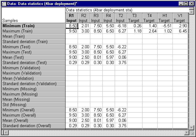
- Click the Data statistics button to review the min, max, mean, and standard deviation of all continuous inputs.
- Notice that the minimum and maximum values from the training data are also included. This information is stored in the PMML file. As always, you should avoid making predictions using inputs that are outside the range of inputs used during training.


Copyright © 2021. Cloud Software Group, Inc. All Rights Reserved.