D-Optimal Split Designs Overview
The standard split plot design is characterized by two sizes of experimental units. Split plot designs began in agriculture where one factor was typically applied to one large plot of land (e.g. fertilizer). This factor was called the whole plot factor. Another factor was applied within the whole plot (e.g. seed variety). This factor was referred to as the sub plot factor. The two experimental units in this case are the whole plot and the sub plot. Since there are two sizes of experimental units, there are two sources of experimental error. This extra source of error affects the subsequent hypothesis tests that are performed.
Split plot designs extend beyond the agricultural setting from which they were originally conceived. It is quite common to encounter these designs in an industrial setting where an experimenter has two factors, where one is considered hard to change and the other is a factor that is easy to change. The hard to change factor may not be reset every experimental run due to complications, whereas the easy to change factor is reset every run.
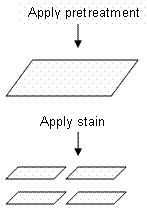
The following illustration comes from Kowalski and Potcner (2003). Consider an experiment where you are trying to determine the water resistance property of wood. There are two factors that are considered: pretreatment and stain. There are two types (levels) of pretreatment and four types (levels) of stain that can be applied to the wood. It is easiest to randomly apply the pretreatments to a whole board and then divide the board into four individual pieces. The stain is then randomly applied to each individual piece. Due to the different levels of randomization there are two distinct sizes of experimental units, the board and the individual pieces. Since there are two different sizes of experimental units there are two sources of error.
Split plot designs can be analyzed in Statistica using either Variance Estimation and Precision or GLM. Variance Estimation and Precision offers two methods of parameter estimation:
REML is a newer method that is now typically recommended to analyze these designs as well as other more general mixed models (i.e. models that contain both random and fixed effects). GLM offers the traditional ANOVA approach only. See Analyzing Designs with Random Effects Using GLM vs. Variance Estimation and Precision for more details.