Example 2: Variance Component Estimation for a Four-Way Mixed Factorial Design
- Specifying the Design
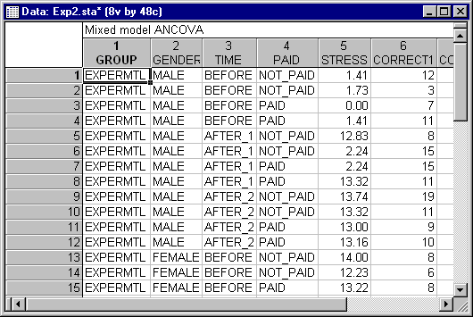
- This example illustrates maximum likelihood (REML and ML) estimation of variance components for a four-way mixed factorial design with multiple dependent variables. The example is based on a data set with four independent variables, a covariate, and three dependent variables. Two of the independent variables, Group and Gender, and their interaction are considered to have fixed effects. The remaining two independent variables, Time and Paid, and their interaction are considered to have random effects. All other interactions involving either Time or Paid are considered to be random effects. The Group and Gender factors have equal N's at each of their two levels. There are unequal N's for Time, with three levels, and Paid, with two levels. The data are contained in the file exp2.sta (a partial listing of this data file is shown below). Open this data file via the File - Open Examples menu; it is in the Datasets folder.
We will first perform the analysis without including the covariate in the model. To specify the design, select Variance Components from the Statistics - Advanced Linear/Nonlinear Models menu to display the Variance Components & Mixed Model ANOVA Startup Panel. On the Quick tab, click the Variables button to display the standard variable selection dialog. Here, select variable Correct1, Correct2, and Correct3 as the Dependent vars, variable Time and Paid as Random factors, variable Group and Gender as Fixed factors, and then click the OK button. By default, a full factorial design will be created, with the Group by Gender interaction treated as a fixed effect and all other interactions treated as random effects, so click the OK button on the Startup Panel to display the Variance Components and Mixed Model ANOVA/ANCOVA Results dialog.
Reviewing the Results.
- Estimation of Variance Components - REML estimation
- To perform REML variance component estimation for the first dependent variable, first click on the
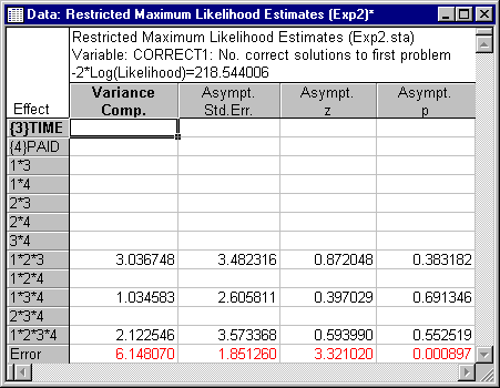
Advanced tab. Then, click the Dependent variables button to display the standard variable selection dialog. Here, select Correct1 as the variable to be analyzed and then click the OK button. Next, select the REML option button under Method, and click the Summary: Components of variance button to display the Restricted Maximum Likelihood Estimates spreadsheet. The variance component estimates, along with asymptotic (large sample) tests of significance, are displayed in the spreadsheet shown below.
To perform the same analysis but with the covariate included in the model, return to the Variance Components & Mixed Model ANOVA Startup Panel by clicking the Cancel button on the Results dialog. Click the Variables button to again display the standard variable selection dialog (your previously chosen variables will still be selected) and then select Stress as the Covariates and click the OK button. Next, click the OK button on the Startup Panel to display the Variance Components and Mixed Model ANOVA/ANCOVA Results dialog. Once again, on the Advanced tab, click the Dependent variables button and select Correct1 as the variable to be analyzed. Make sure that the REML option button is selected under Method, and click the Summary: Components of variance button to display the Restricted Maximum Likelihood Estimates spreadsheet. The variance component estimates, along with asymptotic (large sample) tests of significance, are displayed in the spreadsheet shown below.
Comparing these results to those in the previous spreadsheet, where the covariate was not included in the model, has produced some notable differences. The negative of the natural logarithm of the likelihood decreased when the covariate was included in the model, indicating improvement of fit (the likelihood of the data can vary from zero to one, so minimizing the negative of the natural logarithm times the likelihood of the data amounts to maximizing the probability, or the likelihood, of the data). The estimate of the variance component for Error decreased when the covariate was included in the model, and the estimates of the other nonzero variance components increased. This shows the effects of reduction of the error on the estimation of variance components and the overall fit of the model.
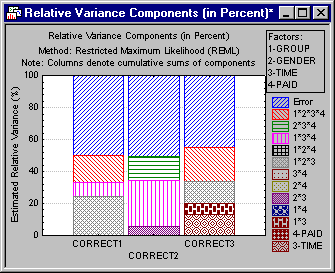
To graphically compare the relative variance components for all three dependent variables, click the Dependent variables button on the Advanced tab and select Correct1, Correct2, and Correct3 as the variables to be analyzed. Then select the Plot relative variances (% of total) check box and click the Stacked bar plot button. This will produce a stacked bar graph which allows you to compare the magnitude of the nonzero variance components for each dependent variable.
- ML estimation
- To perform ML variance component estimation for just the first dependent variable, return to the
Advanced tab, click the Dependent variables button and select Correct1 as the variable to be analyzed. Then, select the ML option button under Method, and click the Summary: Components of variance button to display the Maximum Likelihood Estimates spreadsheet. The variance component estimates, along with asymptotic (large sample) tests of significance, are displayed in the spreadsheet shown below.
Comparing these results with the previous REML estimates, we see that the ML variance component estimate for the Group by Time by Paid interaction effect (1*3*4) is zero. This interaction had the smallest of the nonzero REML variance component estimates.
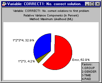
Now we will graphically compare the relative variance components for all three dependent variables using multiple pie charts. On the Advanced tab, click the Dependent variables button and select Correct1, Correct2, and Correct3 as the variables to be analyzed. Then select the Plot relative variances (% of total) check box and click the Pie chart button. This will bring up three pie charts showing the nonzero relative variance components for each of the three dependent variables, allowing you to compare variance components across dependent variables. The pie chart for Correct1 is shown below.
- Summary
- This example has shown how to estimate variance components for complex mixed-model designs. Variance components were estimated for a four-way mixed factorial design. A covariate was also added to the model, to show the effects of reduction of error on the estimates of variance components. Graphical options were also described that aid in the comparison of variance component estimates across multiple dependent variables. Similar results were produced by REML and ML estimation of the variance components.
Implementation of maximum likelihood estimation algorithms is difficult (see, for example, Hemmerle & Hartley, 1973, and Jennrich & Sampson, 1976, for descriptions of these algorithms), and faulty implementation can lead to variance component estimates that lie outside the parameter space, converge prematurely to nonoptimal solutions, or give nonsensical results. Milliken and Johnson (1992) noted all of these problems with the commercial software packages they used to estimate variance components. In the Variance Components and Mixed Model ANOVA/ANCOVA module, care has been taken to avoid these problems as much as possible. Note, for example, that for the analyses reported in this example, most statistical packages do not give reasonable results.
See also Variance Components Index.


