Bayesian Reliability Optimization for Continuous Response Example
Overview
The Bayesian Reliability Optimization for Continuous Response node allows you to obtain the optimized Bayesian reliability (posterior probability of obtaining a pre-defined desirability) over the input space. The key advantage of the Bayesian formulation is that it explicitly takes into account the correlation structure of the data, the variability of the process distribution, and the model parameter uncertainty. The use of a non-informative prior distribution enables a fast, closed form computation of the posterior distribution.
In the example used by Derringer and Suich (1980), the problem is to find the most desirable tire tread compound. In this example, the four Y variables are PICO Abrasion Index, 200 percent modulus, elongation at break, and hardness. The characteristics of the product in terms of the response variables depend on the ingredients, which are the X variables: hydrated silica level, silane coupling level, and sulfur. The goal of the analysis is to find the levels of the ingredients that produce the most desirable tire tread compound in terms of the four outcome measures.
Specifying the Analysis
Derringer and Suich (1980) used a central composite (response surface) design to investigate the effects of the tire tread ingredients on the desirability of the product. The data for the completed experiment of 20 runs (as listed on p. 217 of Derringer Suich, 1980) are contained in the example data file Tiretre.sta.
First, open the Tiretre.sta data file and the Bayesian Reliability Optimization for Continuous Response node:
- On the Datamining tab, in the Tools group, select Workspaces/ Example Procedures.
- When the Select Data Source dialog box displays in a new Workspace, select the Files button, navigate to the file and select it (Program Files>Statistica>Statistica 13>Examples>Datasets> Tiretre.sta). The Dataset icon will display on the Workspace
- The Example Custom Procedures tab now displays on the Statistica toolbar under the Workspace tab.
- Ensure that the Dataset icon is still selected in the Workspace, and double click Bayesian Reliability Optimization for a Continuous Response.
- When the node displays in the Workspace, connected to the Dataset, close the selection box. If the two nodes are not connected, right-click on the dataset and select New Connection from This Node.. and drag the connection to the analytic node.
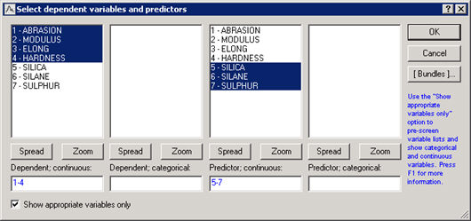
- On the node workspace, double click on the Input Data icon to display a Select dependent variables and predictors dialog box.
- Select the Variables button.
- Specify Abrasion, Modulus, Elong, and Hardness, as the continuous dependent variables in the first selection column.
- Specify Silica, Silane, and Sulfur as the continuous predictor variables in the third selection column.
- Select OK, then OK again to exit the selection dialog box.
| The node allows up to second-order designs. Main effects, quadratic terms and two-way interactions can be included in the design. |
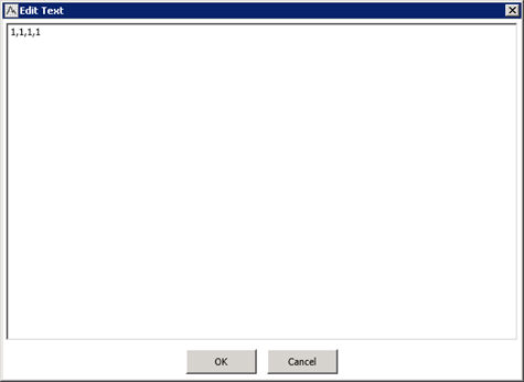
| NOTE: In this example, all first and second order terms will be included in the model. The node automatically includes the main effects in the design. Only the higher order terms need to be specified as a comma separated list. |

| The main purpose of this node is to find the point in the input space that maximizes the posterior probability of the form Pr(D(Y)≥D^* |x), where D^* is the minimum desirability threshold. The node uses a Monte-Carlo estimate of this probability since direct computation will be comparatively slow. |
-
- For this example. leave the box Number of simulations determined by node checked (default) to let the node use a smart default for approximation of the posterior probability. To use your own custom number of simulations, un-check this box and change the number in the Number of simulations numeric input box.
-
- This node provides three different methods to optimize the posterior probability. They are
Numerical search,
Grid search, and
Random search. For this example, the use
Numerical search.
- Numerical search: Uses the L-BFGS-B optimization technique in the Optim package in R.
- Random search: Finds the optimal point by randomly selecting points (by default 3,000) in the factor space. The number of random searches can be specified on the Random search tab.
- Grid search: The node will divide each factor into a grid of equally spaced intervals (by default 4 grid points are used) and will perform the optimization search over the grid.
- This node provides three different methods to optimize the posterior probability. They are
Numerical search,
Grid search, and
Random search. For this example, the use
Numerical search.
| The purpose of the node is to find the design point that maximizes the desirability function being greater than some specified threshold, that is, Pr(D(Y)≥D^* |x), where D^* is the minimum desirability threshold. |
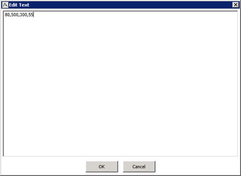
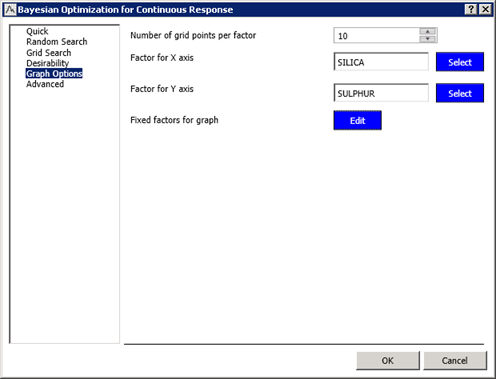
| The node produces graphical output that can help visualize the probability surface as a function of the input factors. Graphical options can be specified on the Graph Options tab. For this example, you will plot the probability as a function of Silica and Sulphur while holding Silane to its maximum value of 1.633. |

Run the node to generate the results. You can monitor the process by watching the bottom status bar. It may take several minutes. When finished, Reporting document will display in the workspace.
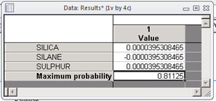
The reporting documents will contain data results displaying the optimal design point found based on the numerical search method along with the value of the maximum probability.
The output also produces the Bayesian reliability graphs for Silica and Sulphur where the third factor Silane is set to maximum value.

This example illustrates the simultaneous optimization of several response variables by means of Bayesian reliability, which, unlike standard frequentist approaches, captures the covariance structure between the responses and addresses parameter uncertainty. It optimizes the posterior probability through a moderately fast computation and also allows you to graphically interpret the design over different factors.