Batch (ByGroup) Analysis Example

The data set

For this example, we will use the classic Iris data file, which contains information about three different types of Iris flowers - Iris SETOSA, Iris VERSICOL, and Iris VIRGINIC. The data set contains measurements of four variables (sepal length and width, petal length and width). The Iris data set has a number of interesting features:

1. One of the classes (SETOSA) is completely separable from the other two (VERSICOL and VIRGINIC).
2. There is some overlap between VERSICOL and VIRGINIC classes.
3. There is some redundancy in the four predictor variables, so it is possible to construct a classification model of the Iris data set using only three of them.

   Objective

It is the goal of this example to draw the above conclusions from the study of the Iris data set using the statistics and graph tools available via Statistica Batch (ByGroup) Analysis.

Open data set/start analysis

Open the example data file IrisSNN.sta, and start the Batch (ByGroup) analysis. Following are instructions to do this from the ribbon bar and from the classic menus.

Ribbon bar. Select the Home tab. In the File group, click the Open arrow and from the drop-down list select Open Examples to display the Open a Statistica Data File dialog box. Double-click the Datasets folder, and then open the data set.

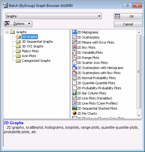
Next, on the Graphs tab, in the More group, click Batch (By Group) to display the Batch (ByGroup) Graph Browser.

Classic menus. Open the data file by selecting Open Examples from the File menu to display the Open a STATISTICA Data File dialog box. The data file is located in the Datasets folder.

Then, from the Graphs menu, select Batch (ByGroup) Analysis to display the Batch (ByGroup) Graph Browser.

To begin with (phase one), we will run some exploratory data analysis tests on the data set. In particular, we want to graphically inspect the separability of data cases belonging to various class memberships and examine the existence of a relationship between the predictor variables. In the second phase, we will build a regression model predicting PWIDTH from the rest of the predictor variables SLENGTH, PLENGTH, and SWIDTH.

Choosing the Graph node

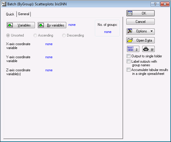
In the Batch (ByGroup) Graph Browser, click the 3D XYZ Graphs folder in the left pane to display its contents in the right pane. Select Scatterplots in the right pane, and click the OK button to display the Batch (ByGroup): Scatterplots dialog box.

Although we would ideally want to view all variables in one graph, this is not possible given that there are a total of four predictors and one independent variable. We will, therefore, generate a sequence of 3D graphs each involving two predictors at a time.

Selecting variables

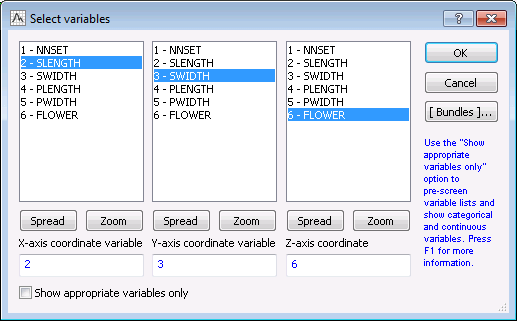
Just as in any STATISTICA analysis, we need to select variables before beginning any calculations. On the Quick tab of the Batch (ByGroup): Scatterplots dialog box, click the Variables button to display a three-column variable selection dialog box. Clear the Show appropriate variables only check box if it is selected in order to display all variables in the data set in the variables lists. Select SLENGTH, SWIDTH, and FLOWER as the x, y, and z-axes, respectively.

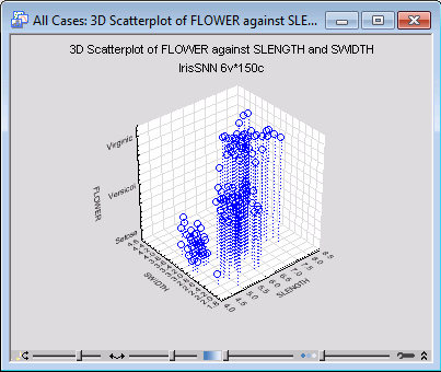
Click the OK button in the variable specification dialog box, and in the message dialog box about text labels, click the Continue with current selection button. Click OK in the Batch (ByGroup) Scatterplots dialog box to generate a 3D graph.

Repeat the above steps for various combinations of SLENGTH, SWIDTH, PLENGTH, and PWIDTH, as the x and y axes, with FLOWER fixed as the z-axis.

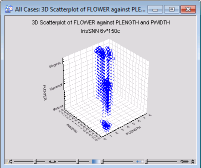
X-axis = PLENGTH and Y-axis = PWIDTH:

X-axis = SLENGTH and Y-axis = PLENGTH:

Compare the graphs we have generated and note that, although there is some overlapping between classes VERSICOL and VIRGINIC, Iris type SETOSA is well separated from the rest. From this we can conclude that, while perfect classification of SETOSA can be achieved using a suitable classifier model, no such separation between VERSICOL and VIRGINIC is generally possible.

So far we have visually analyzed the data and found, from our inspections, that category SETOSA is well separated from VERSICOL and VIRGINIC, while there is some overlap between the latter two. In the next phase of our analysis, we will examine whether there is any redundancy in the predictor variables by building a regression model that can predict PWIDTH from values of SLENGTH, SWIDTH, and PLENGTH. We begin our examination by obtaining estimates of the correlation coefficients between PWIDTH and the rest of the predictor variables on a by-group basis.

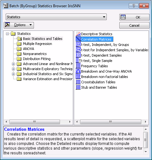
Ribbon bar. Select the Statistics tab. in the Tools group, click Batch By Group to display the Batch (ByGroup) Statistics Browser.

Classic menus. Select Batch (ByGroup) Analysis from the Statistics menu to display the Batch (ByGroup) Statistics Browser .

In the left pane, select the Basic Statistics and Tables folder to display its contents in the right pane. Select Correlation Matrices in the right pane.

Click OK to display the Batch (ByGroup): Correlation Matrices dialog box.

On the Quick tab, click the Variables button to display a variable selection dialog box, and  from the first list select the analysis variables as SLENGTH, SWIDTH, PLENGTH, and PWIDTH. Don't select any variables from the second list. Click OK to accept the selection, close the dialog box, and return to the ByGroup: Correlation Matrices dialog box.

So far we have analyzed the data using the overall data set (i.e., using all cases in the data set). A more categorized inspection is also possible using the by-group feature of the StatisticaBatch (ByGroup) Analysis. Here, instead of using the overall data set, we can analyze data cases belonging to SETOSA, VERSICOL, and VIRGINIC one at a time. In other words, we repeatedly generate results against the set of categories of the variable FLOWER. This can be done by selecting by-group variable(s). Generally speaking, by selecting a by-group variable containing, say, classes A and B, we in effect partition the data cases into two groups (samples). Any analysis conducted on the data set will then be separately applied to each group and the results will be displayed accordingly. Note that we can have more than one bygroup variable at a time.

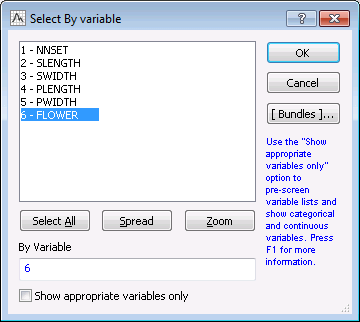
Click the By Variables button in the Batch (ByGroup): Correlation Matrices dialog box to display a single variable selection dialog box. Select FLOWER as the bygroup variable.

Click the OK button. Note that the calculated number of categories found in the bygroup variable is now displayed in the No of groups box (3 in this case, indicating that the by-group variable consists of three categories, namely SETOSA, VIRSICOL, and VIRGINIC).

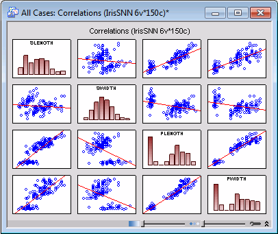
Select the General tab, and set Detail of computed results reported to All results. By selecting this option, the program will produce not only spreadsheets of the correlation coefficients but also 2D scatterplots of the predictor variables together with their individual histograms.

Click the OK button in the Batch (ByGroup): Correlation Matrices dialog box to generate the correlation spreadsheets for the class categories of the by-group variable FLOWER.

An examination of the individual spreadsheets shows that there is some correlation between PWIDTH and the rest of the predictor variables. The strength of these correlations, however, vary from one class to another, but none seems to be substantial, which might indicate that PWIDTH may not so strongly be related to the rest of the predictor variables. This, however, is not the case and can be demonstrated by applying the same analysis, i.e., measurement of the correlation coefficients, using the overall data set.

To do so, click the By Variables button once again on the ByGroup: Correlation Matrices dialog box - Quick tab, cancel the selection of FLOWER as the by-group variable (delete the 6 in the By Variable box at the bottom of the dialog box), and click the OK button.

Click the OK button in the Batch (ByGroup): Correlation Matrices dialog box to run the analysis. An examination of the correlation between PWIDTH and the rest of the predictor variables will show considerable improvement this time, thus providing us with sufficient reason to believe that PWIDTH can be sufficiently modeled using SLENGTH, SWIDTH, and PLENGTH. A visual inspection of the scatterplot graphs confirms this finding.

Our next step is to build a regression model for predicting PWIDTH from the rest of the predictor variables. Click the Cancel button in the Batch (ByGroup): Correlation Matrices dialog box. In the Batch (ByGroup) Statistics Browser, select the Multiple Regression folder and in the right pane, select Standard Multiple Regression. Click OK to display the Batch (ByGroup): Standard Multiple Regression dialog box.

Click the Variables button to display the variable selection dialog box. Select PWIDTH as the Dependent variable; SLENGH, SWIDTH, and PLENGTH as the Continuous predictors; and click the OK button.

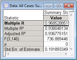
Now we are ready to build a regression model that predicts PWIDTH from the rest of the predictor variables. Click OK to run the analysis and display the results.

Examine the Summary Statistics spreadsheet, and note that the value of R2 is 0.9380. The fact that R2 is close to unity indicates a good regression model, i.e., a regression that can predict the dependent variable with good accuracy from the predictor variables. Note that further examination of the regression model is possible using other properties of the model, including p-value, standard error, and estimates of model coefficients.

See also the Batch (ByGroup) Analysis Index and Browser.