Example 2: Comparing Historical Stock prices

This step-by-step example illustrates how the STATISTICA Extract, Transform, and Load (ETL) module handles stock-related data sets with different time intervals.

Data Sets: Stocks are bought and sold at varying prices throughout each day. Microsoft (ticker MSFT) and Oracle (ticker ORCL) are software companies that trade on the NASDAQ electronic stock exchange. For this example, compare data sets containing historical stock prices with different date/time stamps. The first set contains daily Microsoft price quotes from NASDAQ, while the second set contains weekly Oracle price quotes from another source.

Procedure

  1. From the File menu, select Open Examples
  2. Double-click on the Datasets folder, and open files MicrosoftPrices.sta and OraclePrices.sta into the STATISTICA workspace as the active data sets
    Both data files contain the following columns (variables):
    • DATE - The day on which a trade takes place
    • OPEN - Opening price for the day; first trade of the day
    • HIGH - The highest price of the day
    • LOW - The lowest price of the day
    • CLOSE - Closing price for the day; last trade of the day
    • VOLUME - The daily number of traded shares of a security

    However, they have different date ranges:

    • Microsoft: 10/22/2007-01/04/2008
    • Oracle: 10/18/2007-12/28/2007

    In order to compare the data, the ranges need to be aligned.

  3. To start the analysis, select STATISTICA Extract, Transform, and Load (ETL) from the File > Get External Data submenu
  4. Choose the Time-Indexed submenu to display the STATISTICA Extract, Transform, and Load (ETL): Time-Indexed dialog box, which has three tabs: Quick, Advanced, and Options
    The Quick tab displays the most commonly used options for Time-Indexed STATISTICA ETL
  5. Select the Advanced tab to display options from the Quick tab plus other less commonly used options
    At the top of the Advanced tab, you can select data sources and their associated properties. At the bottom, select the aggregation interval that will be applied globally to all defined data sources.
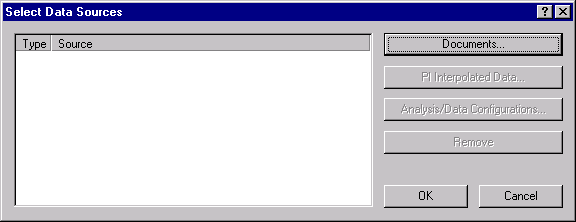
  6. Click the Add data source button to display the Select Data Sources dialog box
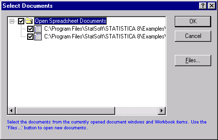
  7. Click the Documents... button to display the Select Documents dialog box. Select the Open Spreadsheets Documents checkbox to select both data files MicrosoftPrices.sta and OraclePrices.sta.
  8. Click the OK button.
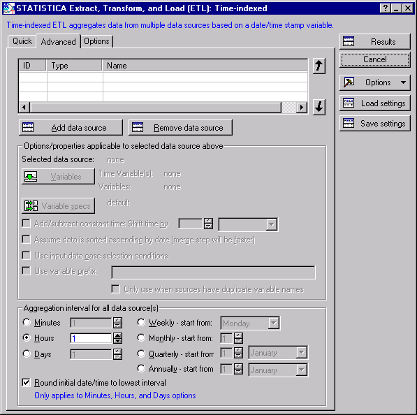
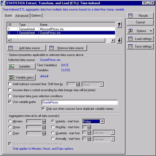
  9. On the Select Data Sources dialog box, click the OK button, and the STATISTICA Extract, Transform, and Load (ETL): Time-indexed dialog box appears as shown below:
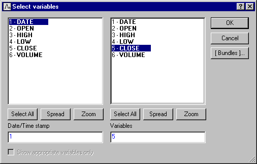
  10. Select MicrosoftPrices.sta from the file list at the top of the dialog, and click the Variables button to display the Variable Selection dialog. Select DATE for the Date/Time stamp; select CLOSE for the Variables.
  11. Click the OK button to close this dialog and return to the STATISTICA Extract, Transform and Load (ETL): Time-indexed dialog box.
  12. Now select OraclePrices.sta from the file list
  13. Click the Variables button, and select variable 1 from the Date/Time stamp list and variable 5 from the Variables list
  14. Click the OK button
  15. In the Aggregation interval for all data source(s) group box, select the Weekly option button, and change the start from field to Friday
  16. For additional date/time options, select the Options tab
  17. Select the Filter all input data sources by the following Date/Time check box
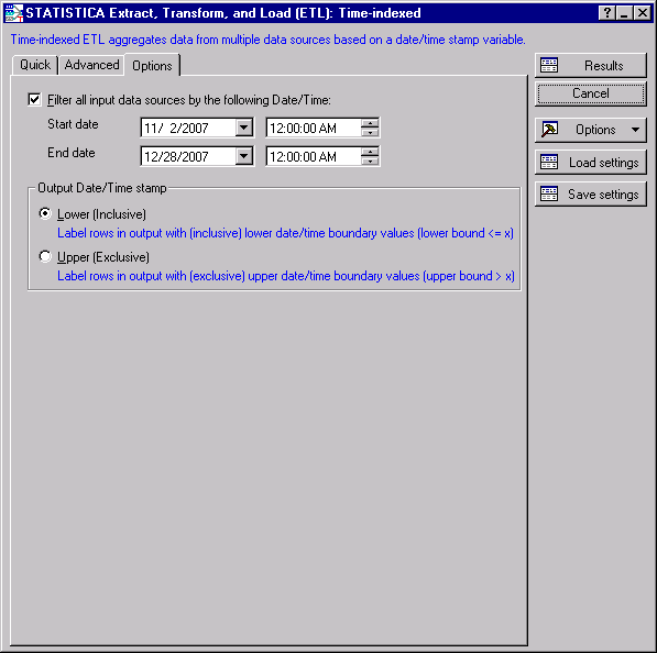
  18. To limit the data that is returned from both selected data files, select 11/2/2007 for the Start date and 12/28/2007 for the End date

    This returns nine weeks of data (Friday to Friday).

  19. Click the Results button to merge the data into a spreadsheet to review result

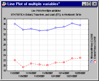
    The two data files are now aligned weekly by date for the range 11/2/2007 to 12/28/2007. The daily closing Microsoft prices are aggregated as means, while the weekly closing Oracle prices are unchanged.

    The Results spreadsheet displays date/time stamps as cases names so that they can be used for graphing the aggregated and aligned data.

  20. From the Graphs > 2D Graphs submenu, select Line Plots (Variables) to display the 2D Line Plots - Variables dialog box
  21. Click the Variables button to display the Select Variables dialog
  22. Select variables 2 and 3, and then the OK button
  23. In the 2D Lineplots - Variables dialog box, select Multiple for the Graph type, and click the OK button.
    Here is the resultant graph plotting Microsoft and Oracle prices