Support Vector Machine Example 1 - Classification
In this example, we will study a classification problem, that is, a problem with a categorical dependent variable. Our task is to build a classification Support Vector Machine (SVM) model that correctly predicts the class label (categories) of a new independent case.
For the example, we will use the classic Iris data set, which contains information about three different types of Iris flowers - Versicol, Virginica, and Setosa. The data set contains measurements of four variables - sepal length and width (SLENGTH and SWIDTH) and petal length and width (PLENGTH and PWIDTH). The Iris data set has a number of interesting features:
Procedure
- One of the classes (Setosa) is linearly separable from the other two. However, the other two classes are not linearly separable.
- There is some overlap between the Versicol and Virginic classes, so it is impossible to achieve a perfect classification rate.
Result
- Data file
- Open IrisSNN.sta; it is in the /Example/Datasets directory of STATISTICA.
- Starting the analysis
- From the Data Mining menu, select Machine Learning (Bayesian, Support Vectors, Nearest Neighbor) to display the Machine Learning Startup Panel. Select Support Vector Machine and click the OK button to display the Support Vector Machines dialog.
- Analysis settings
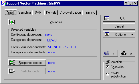
- On the
Quick tab, click the Variables button to display a standard variable selection dialog. Select FLOWER as the Categorical dependent variable and variables 2-5 as the Continuous predictors (independent) variable list, and click the OK button.
At this stage, you can change the specifications of the analysis, e.g., the sampling technique to be used for dividing the data into train and test samples, the SVM and kernel types, etc. Note that some of these analysis settings are not available until the variables are selected.
One important setting to consider is the sampling technique for dividing the data into examples and testing samples (on the Sampling tab). Although the choice of a sampling variable is not the default setting (as a sampling variable may not be available in your data set), you may want to use this option since, unlike random sampling, it divides the data deterministically, which enables you to compare results obtained with various experimental settings. It is recommended that you always provide a test sample as a means of testing the performance of an SVM model when presented with unseen data.
To use a sampling variable for dividing the data, select the Sampling tab. In the Sampling group box, select the Use sample variable option button. Then click the Sample button to display the Sampling variable dialog. Click the Sample Identifier Variable button to display the Cross-Validation Specifications dialog, select NNSET, and click the OK button to return to the Sampling variable dialog. In the Status group box, select the On option button. Next, double-click in the Code for analysis sample field to display the Variable code dialog, select Train as the training sample identifier (cases belonging to Train will be used as the training sample to fit the SVM model), click the OK button to return to the Sampling variable dialog, and click the OK button here to return to the Support Vector Machines dialog.
Now, display the Cross-validation tab and select the Apply v-fold cross-validation check box. Since the selected SVM model is Classification Type 1 (selected by default on the SVM tab) only the Capacity constant is applicable to the analysis. Leave the rest of the options at default, and click OK to initiate SVM training (model fitting), which is carried out in two stages. In the first stage, a search is made for an estimate of the capacity constant that achieves the highest classification accuracy. In the second phase of training, the estimated value of capacity is used to train an SVM model using the entire training sample. When training is finished, the Support Vector Machine Results dialog is displayed.
- Reviewing results
- Use the
Results dialog to review the results of SVM training as well as predictions in the form of spreadsheets, reports, and graphs.
In the Summary box at the top of the Results dialog, you can view specifications of the SVM model, including the number of support vectors and their types, and the kernels and their parameters. Also listed are specifications made in the Support Vector Machines dialog including the dependent and independent variable list, and the values of the training constants (capacity, epsilon and nu). Displayed also is the cross-validation results (when applicable) as well as classification statistics for training, testing, and overall samples (when applicable).
Note. The first thing you should look for on the Results dialog is the cross-validation estimates of the training constants (capacity, epsilon and nu). If any of these values are equal to their maximum cross-validation range, this could be an indication that your search range was not large enough to include the best values. In this cases, click the Cancel button to return to the Support Vector Machines dialog to enhance your search range.
SVM constructs the classification function through a set of support vectors and coefficients. Click the Model button to create spreadsheets of these quantities. This is useful for a detailed review of the SVM model or for inclusion in reports.
Further information can be obtained by clicking the Descriptive statistics button, which will create two spreadsheets containing the classification summary and confusion matrix.
To further view results, you can display the spreadsheet of predictions via the Custom predictions tab (and include any other variable that might be of interest to you, e.g., independent, accuracy, etc., by selecting the respective option button on the Quick tab). You can also display these quantities as histogram plots.
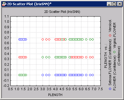
Further graphical review of the results can be made from the Plots tab where you can create two- and three-dimensional plots of the variables and confidence levels. Note that you can display more than one variable in two-dimensional scatterplots.
For example, shown above is a scatterplot of the independent variable PLENGTH against the classification confidence. Note that class Setosa is perfectly separable from Versicol and Virginic, while it is not possible to perfectly distinguish between the latter two (note the region of the x-axis where these two classes significantly overlap, i.e., have similar confidence values). This fact is also reflected in the Predictions spreadsheet created earlier (no miss-classification for Setosa but a noticeable degree of confusion between Versicol and Virginic). To produce the graph shown above, select PLENGTH from the X-axis list and Setosa (conf.), Versicol (conf.), and Virginic (conf.) from the Y-axis list. Then click the Graphs of X and Y button.
Finally, you can perform "what if?" analyses via the Custom predictions tab. You can define new cases (that are not drawn from the data set) and execute the SVM model using them, allowing you to perform ad-hoc, "What if?" analyses. Click the Predictions button to create the spreadsheet of the model.